

Kurtosis is not peakedness - revisited
Kurtosis is not peakedness - revisited
Attempting to parametrise tailedness vs peakedness

Introduction
Until 2014, kurtosis was variously described as a measure reflecting the “flatness”/”peakedness” of a probability distribution relative to the Gaussian (aka Normal) distribution and/or the relative extent of the “tailedness” of the distribution. Voices could be heard for this or for that or for both. In 2014, Westfall published an article strikingly titled “Kurtosis as Peakedness, 1905 – 2014. R.I.P.” In the Summary Westfall states: “Kurtosis tells you virtually nothing about the shape of the peak - its only unambiguous interpretation is in terms of tail extremity; i.e., either existing outliers (for the sample kurtosis) or propensity to produce outliers (for the kurtosis of a probability distribution).”
The purpose of this item is to agree with the first part (virtually nothing about the shape) of Westfall’s summary and to nitpick at the second part (unambiguous interpretation). Kurtosis (as we shall see below) is strongly influenced by tailedness - but it is not silent on peakedness. Shape matters.
The hole in Westfall’s argument
My understanding of Westfall’s argument is that numerically, the centre of a distribution contributes almost nothing to the value of the kurtosis so kurtosis reflects virtually nothing more than the extent of the tails of the distribution. To illustrate this argument Westfall offers (in Figure 2) three distributions with identical value (2.4) for the kurtosis (and a value close to that of the Gaussian distribution, 3). The first is a “flat-peaked” distribution which Westfall calls the “Devils tower distribution”, referring to an American landmark but a South African might prefer to call it the Table Mountain distribution. The second could not have a sharper point (be more peaked), being a triangular distribution. The third is a bimodal distribution, with two unlimited peaks and a centre which is sort an inversion of a peak (it dips where it should be bulging!), which Westfall calls the “slip-dress” distribution. For non-Americans, the pinafore distribution?
Having established a point of reference, Westfall modifies all three distributions in the same way by (in effect) moving some of the distribution out from the body of the distribution into a distant point in the tails either side of the body of a distribution. In technical terms, he creates a mixed distribution for each of the original distributions. If f(x) is one of the original distributions then for another distribution g(x), a mixed distribution is p·f(x)+(1-p)·g(x), 0<p<1. The distribution g(x) Westfall uses (with p slightly less than 1) increase the kurtosis of all three mixed distributions to approximately 6 - but the graph (Figure 3) of the mixed distributions is indistinguishable from the original distributions. Westfall’s presentation is highly technical and inaccessible to the ordinary reader.
The purpose of this post is to point out that values of the distribution within one standard deviation from the mean, µ ± σ, do indeed make little numerical contribution to the even central moments (because raising a fraction to an even power creates a positive amount which is an even smaller fraction) and that values of the distribution outside the the limits of one standard deviation, values exceeding 1, sign ignored, are the ones determining the magnitude of the even central moments. However, the values in the centre of the distribution make a contribution by their presence, by the proportion (probability) of the distribution in the centre. If values in the centre are moved out into the tails of the distribution, the shape of the tails will change - as will the part of the distribution from which values were moved. To be able to see the change in the shape of the distribution one must compare distributions with the same variance (with variance =1 being a useful selection). One can than point at a value µ ± kσ which was moved to µ ± Kσ (K > k) and examine the effect of the move on the value kurtosis and the shape of the distribution, where K and k would be “pure numbers”; not numbers with different interpretations because of different standard deviations.
Simplifying the mathematics
In the first place, I will ignore skew and bimodal distributions. Simply graphing the distribution will reveal such anomalies. Instead, I will limit the discussion to symmetric distributions. Such distributions can be thought of having five parts, a centre and two pairs of mirrored parts, the “shoulders” and the tails, either side of the centre. To avoid advanced mathematics, I will limit myself to a discrete distribution, of x, which has five distinct values.
Left tail: A proportion p of values equal to µ - MS
Left shoulder: A proportion mp values equal to µ - S
Center: A proportion 1-2mp-2p values equal to µ
Right shoulder: A proportion mp values equal to µ + S
Right tail: A proportion p of values equal to µ + MS
The value of S must be greater than 0 and the value of M must be greater than 1. The proportion (or, to give it its technical name, the probability) p must greater than zero (but less than 1) and we require mp ≥ p which simplifies to m ≥ 1. To exclude bimodality, we require 1-2mp-2p ≥ mp which simplifies to p(3m+2) ≤ 1. The value of E[x] is
E[x] =p·(µ - MS) + mp·(µ - S) + (1-2mp-2p)·µ + mp·(µ + S) + p·(µ + MS) = µ.
Defining y = x - µ, the variance of x is equal to E[y²] which we abbreviate to σ². Defining z = y÷σ, the kurtosis is defined to be E[z⁴] = E[y⁴]÷σ⁴. We need to calculate two values, the variance of x, Var(x) and the kurtosis of x, Kurt(x):
E[y²] = p·(-MS)² + mp·(-S)² + (N-2mp-2p)·0² + mp·(S)² + p·(-MS)²
= 2·p·M²S² + 2·mp·S² + 0
= 2pS²[M² + m]
E[y⁴] = p·(-MS)⁴ + mp·(-S)⁴ + (N-2mp-2p)·0⁴ + mp·(S)⁴ +p·(-MS)⁴
= 2·p·M⁴S⁴ + 2·mp·S⁴ + 0
= 2pS⁴[M⁴ + m]
Hence
E[z⁴] = E[y⁴]÷σ⁴ = E[y⁴]÷{σ²}² = {2pS⁴·[M⁴ + m]} ÷ {2pS²·[M² + m]}²
= {2pS⁴}÷{2pS²}²·{[M⁴ + m]÷[M² + m]²}
= {1÷(2p)}·{[M⁴ + m]÷[M² + m]²}
The distribution we’ve defined has five unknowns, µ, S, p, M and m. The first was eliminated because the definition of kurtosis is in terms of y = x - µ. The second cancelled out in the formula for Kurt(x) but it is still present in the formula for Var(x). To convert S into an interpretable value, let’s consider it to be k standard deviations of x, i.e. that the “shoulders” are values k standard deviations from µ. In that case, S = k·√Var(x) or S² = k²·Var(x) = k²·2pS²[M² + m] which simplifies (cancelling S² on both sides of the equation) to 1 = k²·2p[M² + m] or {1÷(2p)} = k²·[M² + m] which leads to the relationship
p = 1÷[2k²·(M² + m)]
so that the requirement p(3m+2) ≤ 1 established above now becomes
(3m+2)÷[2k²·(M² + m)]≤ 1 or, equivalently, k²≥(3m+2)÷[2(M² + m)]
while Kurt(x) simplifies to
Kurt(x) = k²·[M² + m]·{[M⁴ + m]÷[M² + m]²} = k²·{[M⁴ + m]÷[M² + m]}
Setting µ = 0 and writing σ² for Var(x), we can now simplify the distribution we are studying as follows:
Left tail: A proportion p of values equal to -Mkσ
Left shoulder: A proportion mp values equal to -kσ
Center: A proportion 1-2mp-2p values equal to 0
Right shoulder: A proportion mp values equal to kσ
Right tail: A proportion p of values equal to Mkσ
in which p = 1÷[2k²·(M² + m)].
As a check, note that the total of the proportions is p+mp+1-2mp-2p+mp+p=1, E(x)=µ= 0 and Var(x) = p·M²k²σ²+mp·k²σ²+mp·k²σ²+p·M²k²σ² = k²·2p·[M²+m] ·σ² = p·2k²·(M²+m]) ·σ² = σ² while Kurt(x) = [2·p·M⁴k⁴σ⁴+2·mp·k⁴σ⁴]÷[σ²]² = k²·p·2k²·[M⁴+m] = k²÷[2k²·(M²+m)]·2k²·[M⁴+m] = k²·[M⁴+m]÷[M²+m]. Note that the kurtosis is unaffected if x is scaled by a factor - we saw this with S - the factor increased the kurtosis by its fourth power above the line and by the square of a square below the line. As a result, we can eliminate σ in the modified family of distributions by setting σ = 1. In short, it may appear that k is merely S renamed - but k has an interpretation while S does not.
We have described a family of distributions which are characterized by the distance of the shoulders from the centre (k) and the concentration of the distribution in the shoulders (m) relative to the tails, along with the distance of the tails from the centre (M). The idea is that we will select values for k, m and M, that will define the value of p and we’ll be able to calculate the value of the kurtosis for the selected values.
The formula for Kurt(x), k²·[M⁴+m]÷[M² + m], has some obvious implications. For k = 1 and pretending m = 0, the formula simplifies to M² which would be 9 when M=3 (in this case corresponding to three standard deviations from the centre) so it is clearly true that, numerically, the primary determinant of kurtosis is the tailedness of the distribution. However, note that the proportion of the distribution in the shoulders (as determined by m) will tend to reduce the kurtosis. In the case M=3, where one has 81÷9 = 9 when m=0, one has (81+1)÷(9+1) = 8.2 when m=1 and (81+2)÷(9+2)=7.55 when m=2. The maximum valid value for m in this case is 16, in which case the Kurtosis is (81+16)÷(9+16)=3.88. Increasing m, “fattening the peak”, reduces the kurtosis. While M is a major modifier, the effect of m is much milder.
Since the family of distributions is defined by M>1 and m≥1, we can arrive at the conclusions stated above - but care must be taken with k>0. This is because the three parameters M, m and k don’t only determine the values of x, they also determine the proportions of the tail, shoulder and central values. Table 1 offers three distributions. in the family described above, and a fourth which would be a member if one relaxed a requirement for membership. All have M=3 and m=2 but they differ in their value of k (which is displayed in the third column of the table). The distributions are displayed graphically below the table.
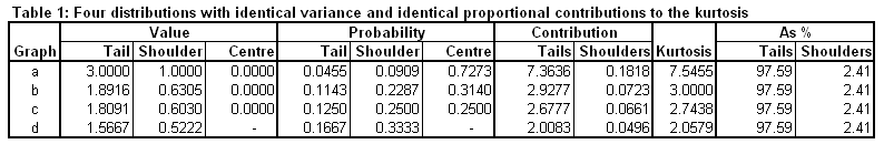
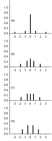
Distribution (a) is the starting point. It is clearly a peaked distribution but is also has outliers - the shoulders are at one standard deviation from the centre and the tails are three standard deviations from the centre - k = 1 for this distribution. The kurtosis is 7.5455, a value 97.59% of which is determined by the tails, the remaining 2.41% being contributed by the shoulders, with the centre contributing nothing to the numerical value of the kurtosis. For Westfall, this makes the case that kurtosis is tailedness, not peakedness.
In my opinion, Westfall is failing to notice that the centre is contributing to the value of the kurtosis indirectly, through having the probability concentrated in the centre. In our initial distribution, 72.73% of the probability is concentrated at the centre. Let’s explore what happens if we reduce the concentration in the centre. If we change the shape of the distribution while keeping the variance equal to unity and the contributions at 0.9759:0.0241 we can solve for k in the formula for the kurtosis above when setting that value to 3, distribution (b) in the table and graph:
k²·{[M⁴ + m]÷[M² + m]} = 3 implies that k is the square root of
3·{[M² + m]÷[M⁴ + m]} = 3·{[9 + 2]÷[81 + 2]} = 33÷83 which yields k = 0.6305.
This exercise is intended to demonstrate that reducing the tailedness and the peakedness of a distribution - by changing the shape of the distribution in a controlled fashion - the result will be a reduction of the kurtosis.
Reducing k from unity to the new value also changes the probabilities. In the tails we have 1÷[2k²·(M² + m)] = 1÷[2·(33÷83)·(9+2)] = 83÷(2·33·11) = 83÷726 = 0.1143 and in the shoulders we have (by choice) twice that value. The value in the shoulders is k and the values in the tails is (by choice) three times that amount.
We can continue down this road, making the probability of the centre be the same as in either shoulder, distribution (c) in the table and graphs, yielding a kurtosis of 2.7438. We can even remove the centre, distribution (d) in the table and graphs, from the distribution, as long as this is done in a manner to keep the variance at unity and the proportional contributions to the kurtosis at 0.9759:0.0241. Even though this fourth distribution is not a member of the family described above (strictly, it would be bimodal if it were), it still has unit variance and the contributions to the kurtosis (2.0579) is still 0.9759:0.0241 from the tails and shoulders respectively. It’s important to distinguish this case (one with 4 values) from the case of 5 values where the value at the centre, 0, has a probability of 0. I mean to exclude bimodality. Distribution (d) is meant to be the same as distribution (a) in two crucial aspects - the variance is unity and the proportional contributions of the tails and shoulders to the kurtosis is the same. The distributions are intended to differ only in the excising of the centre. This changes the kurtosis from 7.5455 to 2.0579, making the point that the presence of the centre, the peakedness of the distribution, contributed to the large kurtosis value distribution (a) has, despite the fact that the centre contributed nothing (zero) to the value of 7.5455.
Summary
Westfall summarises his paper with the following paragraph:
“As I have shown, kurtosis tells you very little about the peak or centre of a distribution. Thus, kurtosis should never be defined in terms of peakedness. To do so is counterproductive to the aim of fostering statistical literacy. The relationship of peakedness with kurtosis is now officially over.”
My objection is to the last sentence. It seems to me that kurtosis is dominantly as a result of tailedness - but moving probability out into the tails (to create tailedness) implies that the shape of the centre of the distribution must change to keep the variance constant. Lengthening the tails will increase the variance, so there must be a compensatory “thinning” of the peak, increasing peakedness. In short, I disagree with the statement that there is no relationship between peakedness and kurtosis.
Appendix A
The graphs (distributions) used in the presentation above are a bit “thin” or “spiky” because they are discrete distributions. In this appendix a simple continuous example is presented. The strategy is a little different. In the example following, the values of the distribution are assumed to vary between -3.5 standard deviations and +3.5 standard deviations and they are grouped into 7 groups of length of one standard deviation. In each of the intervals the values are assumed to be equally likely. The probabilities for the values covered by the 7 rectangles are p₄ for the two tails (between -3.5 and -2.5 on the left and +2.5 to +3.5 on the right), p₃ for the next two groups towards the centre, p₂ for the next pair and p₁ for the central group (from -0.5 to +0.5).

The r-th moment is calculated piecewise, for each rectangle, with the contribution from a rectangle being as seen here with the understanding the the value 1÷(b-a) in the link is pₖ in the formula below, for k = 1, 2, 3 and 4. (Please be aware that I’m exploiting the fact that the width of the rectangles is unity; this simplifies the algebra below.) Under the conditions specified, the formua for the rth moment is as follows:
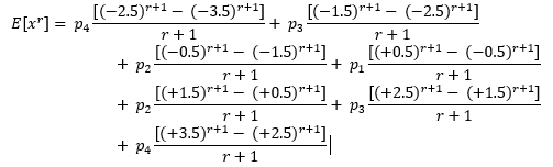
The odd moments are all zero because r+1 is even when r is odd. For example, when r=1, p₄ is multiplied by [(-2.5)² - (-3.5)²] = [(2.5)² - (3.5)²] (and divided by r + 1 = 2) from the left tail but [(+3.5)² - (+2.5)²] = -[(2.5)² - (3.5)²] so these pairs cancel one another out, while, for p₁, [(+0.5)² - (-0.5)²] = [(0.5)² - (0.5)²] = 0.
For r=2 and r=4 the equation simplifies to the following:

These equations can be simplified by introducing the requirement that
p₁+2p₂+2p₃+2p₄ = 1 so that p₁ = 1-2p₂-2p₃-2p₄ which may be substituted into the formulas above, to get:

Next, since E[x] = 0, Var(x) = E[x²] so if we impose the restriction Var(x) = 1, we can solve for p₂ to obtain p₂ = 11÷24 - 4p₃ - 9p₄. Substituting this into the equations above, we get:

Thus Kurt(x) = E[x⁴] = 1.3875 +24p₃ + 144p₄. Our intention is to set p₄ (the probability in either of the two tails, between -3.5 and -2.5 or between +2.5 and 3.5) and then to explore the effect of varying p₃. Since 3 is a point of reference, we can ask what value of p₃ will yield this value for the kurtosis, given the selected value of p₄. The solution is p₃ = 43÷640 - 6p₄.
The requirements p₁ ≥ p₂ ≥ p₃ ≥ p₄ place further restrictions. The first inequality, p₁ ≥ p₂, and the equations above lead to p₃ ≥ 3÷80 - 2.5p₄ so that, this combined with the last inequality, p₃ ≥ p₄, yields p₃ ≥ max(p₄,3÷80 - 2.5p₄). The second inequality, p₂ ≥ p₃, and the equation for p₂ above simplifies to p₃≤11÷120-1.8p₄.
To be able to graph the distributions (the rectangles centred at -3 and +3 have a height of one pixel), I chose p₄ = 0.004 for which the lower bound for p₃ is 11/400 = 0.0.275, the value of p₃ having kurtosis equal 3 is 691÷16000 = 0.0431875 and the upper bound for p₃ is 1267/15000 = 0.08446667. For these three values, the kurtosis is 2.6235, 3 and 3.9907. These three distributions are graphed below.
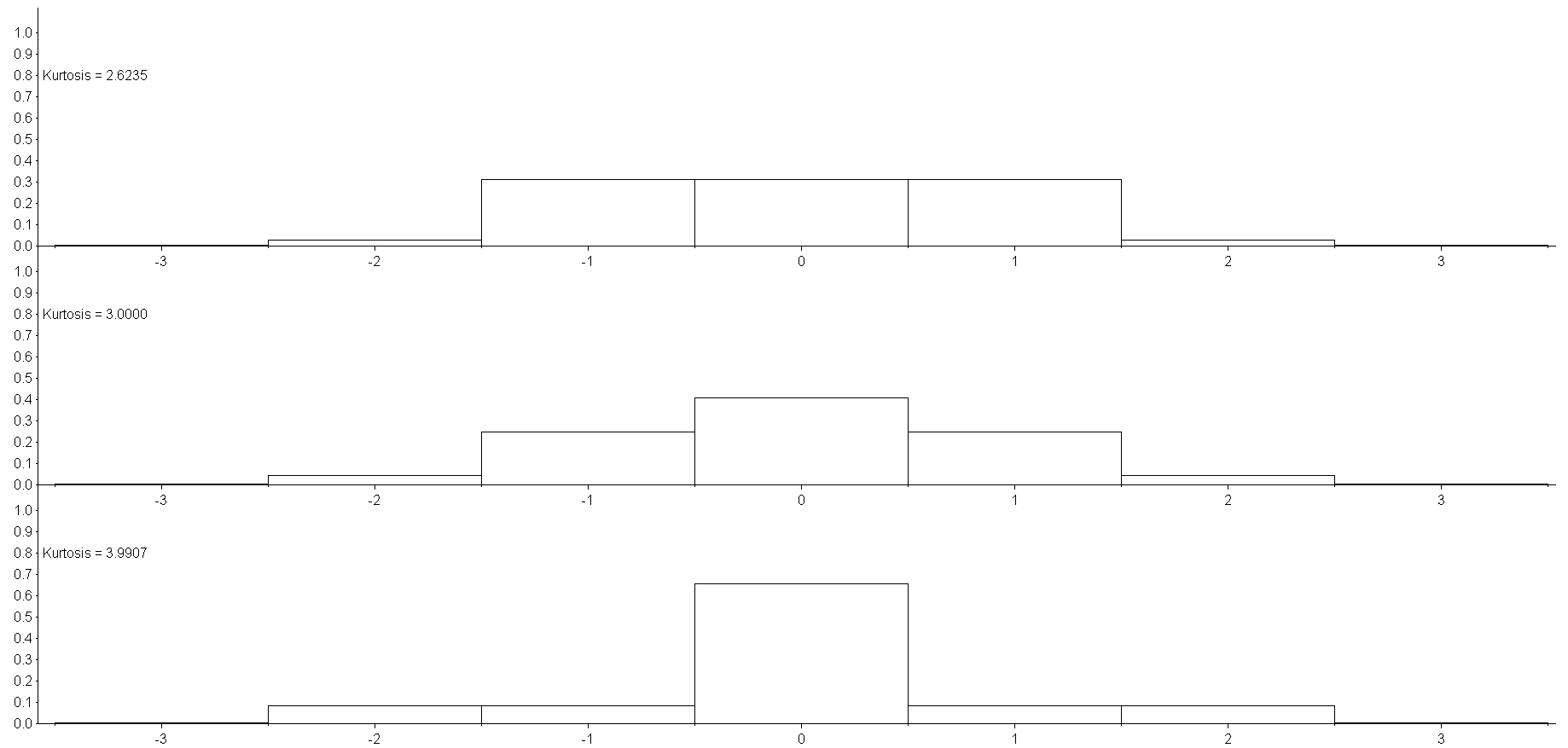
The three distributions have the same tails, p₄ = 0.004, their variances are the same, but their kurtosis has been modified by changing the shape - the peakedness - of the distribution.
Appendix B
This post is an attempt to make a point while keeping the mathematics at the simplest level possible. Fortunately, there are links on the internet which supply us with useful formulas which we do not need to see derived. We hope that when these formulas are used to graph distributions, our point will be made.
Westfall used mixtures of distributions to make his point. In this link we learn that given two Gaussian or Normal distributions, symbolized by x₁ ~ N(µ₁,σ₁²) and x₂ ~ N(µ₂,σ₂²), and a mixture defined by p, 0<p<1, x = p·x₁ + (1-p)·x₂, written
x ~ p·N(µ₁,σ₁²) + (1-p)·N(µ₂,σ₂²),
then the first moment of x is E[x] = p·µ₁ + (1-p)·µ₂ = µ and the variance of x is Var(x) = p·σ₁² + (1-p)·σ₂² + p·[µ₁ - µ]² + (1-p)·[µ₂ - µ]². If µ₁ = µ₂ (= µ), the variance simplifies to Var(x) = p·σ₁² + (1-p)·σ₂² and the kurtosis of the mixture will be
Kurt(x) = 3·[p·(σ₁²)² + (1-p)·(σ₂²)²]÷[{p·σ₁² + (1-p)·σ₂²}²].
i.e. with the µ₁ = µ₂ = µ = 0 the mixture has three parameters, p, σ₁² and σ₂², where the third can be eliminated by requiring Var(x) = 1 (so that σ₂² = [1 - p·σ₁²]÷[1-p] ), then we may compare the mixture to the N(0,1) distribution, which has a kurtosis of 3.
Selecting p = 0.8 and σ₁² = 0.5 we calculate (using the formulas above) that σ₂² = 3 and Kurt(x) = 6. A comparison of the two distributions is shown below:

All the graphs are plotted between -5 and +5 - there are values indistinguishable from zero (the plot of the x-axis) which show up as coloured pixels. Note that most diagrams misrepresent the Normal or Gaussian distribution by (in effect) magnifying the vertical axis relative to the horizontal axis. In the plot above, the same number of pixels are used to represent 0 to 1 horizontally as are used vertically.
The top plot shows the standardized Gaussian distribution (in blue). This distribution is used as a point of reference when evaluating kurtosis. It has a value of 3 for the kurtosis. The second distribution plotted is our mixture of two Gaussian distributions and it has a kurtosis of 6. The third and last plot is of the difference between the two distributions. It shows that the second plot was created by moving values more-less between -2 to -1 and between +1 to +2 to the centre of the distribution, more or less between -1 and +1. Such movement would reduce the variance of the mixed variable - but the compensation is to move values out into the tails of the distribution. Values out at 4 standard deviations from the centre contribute some fraction of 4² = 16 to the variance but the same fraction of 4⁴ = 256 to the kurtosis, so the kurtosis of the mixture distribution is 6. That the larger value for the kurtosis is attributable to the tails is indisputable - but the needed change in the shape of the distribution to achieve these tails should not be summarily dismissed as Westfall does in his paper. This example shows clearly that increased kurtosis is associated with increased peakedness. It cannot be otherwise! It’s a see-saw - if you want things to go up here, things will have to go down there. The shape of a symmetric unimodal distribution with a specified kurtosis is determined by two requirements - the sum of the probabilities (for a discrete distrbution) must equal unity or the area under the curve of the distribution (for a continuous distribution) must equal unity and the variance of the variable must equal unity (which is achievable by standardizing) to establish a single formula for the kurtosis - it is the fourth moment of the standardized variable.
Given a distribution with some value for the kurtosis, that kurtosis can be increased by moving values from the center or shoulders of the distribution towards the tails. Such movement will also increase the variance, so to bring that back to unity, values must be moved from the shoulders towards the center. Increasing the kurtosis of a unimodal symmetric distribution increases the “peakedness” of that distibution.