
How much storage would make wind and PV comparable to nuclear power?
Based on the data for February and March 2024

In a previous post, I examined the performance of “renewables” in South Africa using Eskom’s data for February and March 2024. This dataset supplies the hourly output (24 values per day) for the 29+31 = 60 days in the period, so 1440 values in total for PV and wind output and for the installed capacity of each (2287.09 MW of PV and 3442.57 MW of wind). To eliminate the need to scale graphs, I divided an hour’s output by the installed capacity in that hour, calling this amount the Capacity Factor (CF), which I expressed as a percentage.
PV
To establish what I hoped would be a lower bound for the battery requirements which would ensure a steady output from PV, I averaged over the 60 days in the period for each hour of the day to obtain the values in the first three columns of the table below. Taking the output to be the average over the hours of the day, the value in the “Smoothed” column, I was able to simulate the performance of storage (see the column headed “Battery”). When there’s a shortfall in production, the output must come from the battery (a MW value in each of the 24 hours) and the running total indicates the accumulated charging (positive values) and discharging (negative values) of the battery (a MWh value), as shown in the following spreadsheet:
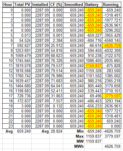
The largest hourly value in the “Battery” column (sign ignored) is 1159.837 MW and the largest accumulated value (again, sign ignored) is 4626.759 MWh. The ratio of these two numbers is 3.989 which is convenient because Li-ion batteries typically have a MWh value 4 times the MW value. The ratio of the installed PV value (2287.09) to 1159.837 is 1.972 which I will round up to 2.
The analysis above suggests that for every 2 MW of PV we require a MW (and 4 MWh) of batteries. I will take the MW value to be 1160 (which is half of 2320, slightly larger than 2287.09) and the MWh value to be 4640.
The following graph plots the average outputs (the horizontal lines) and the daily output from 01/02/204 to 31/03/2024 within each hour; each horizontal line is 60 pixels wide and the “jagged” lines in an hour indicate the variation within an hour.

The unlabelled tick-marks on the x-axis label 14/02/204, 29/02/24 and 15/03/2024 in each hour of the day. As a side note, the pattern in variation between 06:00 and 07:00 (a slope to the right) is mainly because of the change in the time of sunrise in February and March.
Wind
Performing the same calculations for wind as for solar, we find the following:
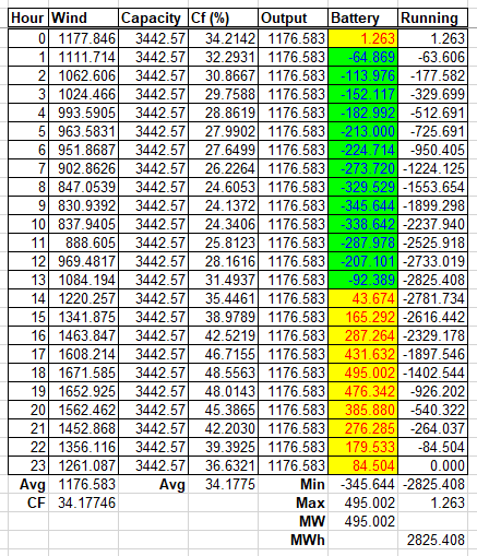
The ratio of 2825.408 to 495.002 is 5.708, so, assuming an upper bound of 4 for this ratio, the MW value must be increased. Setting this to 707, (a MWh value of 2828) the ratio of 3442.57 to 707 is 4.869, which I’ll round to 5.
The analysis suggests that for every 5 MW of wind we require a MW (and 4 MWh) of batteries which I take to be 707 MW (and 2828 MWh).
The graph for wind is very different to the graph for PV.

The pattern in the hourly average is fascinating. At this time of year, from about 11:00 the output picks up steadily, peaking at some time between 18:00 and 19:00, after which there’s a steady decrease to a minium some time between 09:00 and 10:00 the next day. The variability from day to day within the same hour of the day is also remarkable. Please keep in mind that each of the two graphs above can be thought of as 24 adjacent plots of the output at a specified hour for the 60 days of the period. We see that for PV, if the average in some hour is some value, the actual value on a particular day will be close to that average value — but for wind the actual value on a day could be very much further away from the average value on that day. I feel it’s worth quantifying this difference between PV and wind, which is my next step.
A standard ANOVA between and within hours
Faced with variability in a variable y where one has groups and observations within groups, one can calculate the overall mean, m, and an a mean for all the observations for a group, g, there being as many values g as there are groups. We might now consider the deviations y - m. Some kind of average of these deviations would measure the total variability. (Note that the sum of deviations from the mean of the observations is always equal to zero - so it’s not useful to calculate the simple mean of the deviation. One must eliminate the sign of the deviations - and one way to do that is to square the deviation.)
We might then consider partitioning the total variability by introducing the group means, as follows:
(y - m) = [(y - g) + (g - m)]
where the g is used is the g matching the group the observation belongs to. Squaring both sides of the equation we get
(y - m)² = (y - g)² + 2(y - g)(g - m) + (g - m)²
Next totalling both sides, first grouping deviations into their groups, then totalling these group totals, note that in the first step, for each group, the value of (g - m) is the same amount for every (y - g) and the sum of (y - g) is zero for the group - so the sum, for the entire dataset, of (y - g)(g - m), is zero. Hence:
Sum(y - m)² = Sum(y - g)² + Sum(g - m)²
in which the first term on the right sums the variability within groups while the second sums the variability of group means over groups.
We have a means of partitioning total variability into variability within and between groups. Such activities are called “Analyses of Variance” which is abbreviated to ANOVA.
In the current dataset we get the following summary:
We see that:
PV is considerably more variable than wind - the first total is more than 4 times large than the second; what would one expect when the variability in PV of night (0%) versus day (heading to 100% then heading back down to zero) is compared to wind’s more gradual sweep down then up then down again through a day.
The pattern in the variability for PV (the ratio of Between to Within is just over 20) is the opposite of the pattern of variability for wind (the ratio of Within to Between is just over 3)
The pattern in the variability is maintained, even when the total variability is standardized to 100.
Conclusion
I must conclude by emphasizing that the above analysis is an attempt to establish a lower bound to the requirement for storage which would stabilize (smooth) the output from wind and solar. When I used the values calculated and performed the calculations on an hourly basis, I soon discovered that there would be times when production was below the output set and that the batteries had been emptied - so output below the value set would be the only option available - think load shedding. Just so, there would be times when production was so good that the output set was met, the surplus was going to the battery - but either the MW value or the MWh value was exceeded. Curtailment, spillage, wastage would be the only option available.
Note too that I’ve ignored realities such as the loss of energy when there’s a transition from one form to another (this happens in both directions, from electrical to chemical and from chemical to electrical).